Plot/Fit PSI μSR data
The musrfit.cgi script is a web based graphical user interface for plotting and fitting PSI µSR data. The interface acts as a wrapper to the musrfit software and uses many of its capabilities in a user friendly way. However, to utilize the full power of musrfit for we recommend that you either install musrfit locally on your computer or use the software installed on the PSI local computers.
Thank you for using this script. Please contact Zaher Salman <zaher.salman “at” psi.ch> if you have any problems, suggestions or comments.
Setting up the fit
The musrfit.cgi script can be reached using any web browser, also from outside PSI, by following this link
http://musruser.psi.ch/cgi-bin/musrfit.cgi
You will then see the following html form:
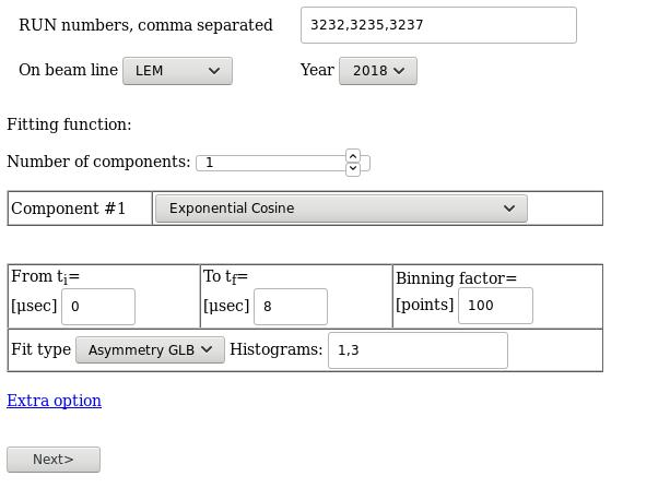
You may initially ignore the “Extra options”. We will return to these later on. To start with you should type the run numbers that you wish to fit. For multiple runs you can use the following (msr2data) notation:
- comma separated run numbers: 3232,3235,3237
- hyphen denotes a series, from-to, i.e. 3232-3234 means 3232,3233,3234
- colon denotes a loop with a step, from:to:step, i.e. 3232:3238:2 means 3232,3234,3236,3238
The script allows you to fit the data to a sum of unlimited number of components. These components can be one of the standard functions already available in musrfit
- Constant Background – Non-relaxing asymmetry
- Exponential – Exponential relaxation function
- Gaussian – Gaussian relaxation function
- Stretch Exponential – Stretched exponential relaxation function
- Exponential Cosine – Exponentially damped oscillation
- Gaussian Cosine – Guassian damped oscillation
- Stretch Cosine – Stretched exponentially damped oscillation
- Lorentzian Dynamic Kubo-Toyabe LF
- Gaussian Dynamic Kubo-Toyabe LF
- Lorentzian Kubo-Toyabe LF x Exp – Lorentzian Kubo-Toyabe LF multiplied by an exponential function
- Gaussian Kubo-Toyabe LF x Exp – Gaussian Kubo-Toyabe LF multiplied by an exponential function
- Lorentzian Kubo-Toyabe LF x Str Exp – Lorentzian Kubo-Toyabe LF multiplied by a stretched exponential function
- Gaussian Kubo-Toyabe LF x Str Exp – Gaussian Kubo-Toyabe LF multiplied by a stretched exponential function
Simply chose the number of components in your fit function and then select a suitable standard function from the corresponding drop-down menu. Components with “None” selected will be simply ignored, however, try to avoid doing that by reducing the number of components.
Next, select the time range for fitting; “ti” and “tf” are the initial and final time, respectively. You may also change the binning factor for the fit. Typically for LEM data one should use 100-200 and for bulk data 10-50.
The “Fit type” drop-down menu allows you to choose the type of fit you are performing, either “Asymmetry”/”Asymmetry GLB” or “Single Hist” fits.
For an “Asymmetry”/”Asymmetry GLB” fit, you must provide only two comma separated histogram numbers in the “Histograms” field. These numbers denote the order of the histograms in the data file and will be used to calculate the asymmetry between them. One very useful option is addition of histograms before calculating the asymmetry. For example, in recent LEM data files the histograms 1 and 5 are the upstream and downstream parts of the left detector respectively, while 3 and 7 are the upstream and downstream parts of the right detector. Therefore, to calculate the asymmetry between left/right detectors one should use “1 5,3 7”, which indicates that the asymmetry will be calculated between the sums of 1+5 and 3+7.
For a “Single Hist” fit, you may put in the “Histograms” field as many comma separated histograms (valid numbers) as you wish. These will be fit assuming that the asymmetry in all these histograms follows the same function, with the exception of the phase if present. The same histogram summation rule above (space separated) applies also here.
What is the difference between “Asymmetry”and ”Asymmetry GLB”? Generally, I would suggest using ”Asymmetry GLB” which utilizes the “global” option built into msr2data in a smart way. Therefore, msr files generated this way will be usable also on your computer for further analysis. The “Asymmetry” produces non-standard msr files created according to Zaher’s warped logic. They can be more flexible, but if you do not miss this flexibility do not even go there.
Now, we return to the “Extra option”, which allow the user to change the title which will be included in the msr file and the name of the generated msr file. Both are optional, if left empty, the script will use the title of the first run and a standard file name RUN_BEAMLINE_YEAR, where RUN is the first run number, BEAMLINE and YEAR are the values from the corresponding drop-down menus.
Finally, you may proceed to the next fitting stage by clicking the “Next>”.
Shared fit parameters
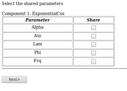
This stage will be available only when you are performing a fit which includes multiple runs, i.e. you had more than one run number in the “RUN numbers” field. Here, you will be able to tell musrfit which parameters are to be shared among all runs by selecting the corresponding check box of the parameter (see figure below). Then you may proceed to the next step by clicking “Next>”.
Plot/fit iterations
Finally, you reach the most important stage in the fitting procedure. Initially, using default parameters, the script will plot the requested data. You will be able to see how good you initial guess is and adjust it before you try to properly fit the data. This can be done in the editable parameters table shown below the plot (see figure below).
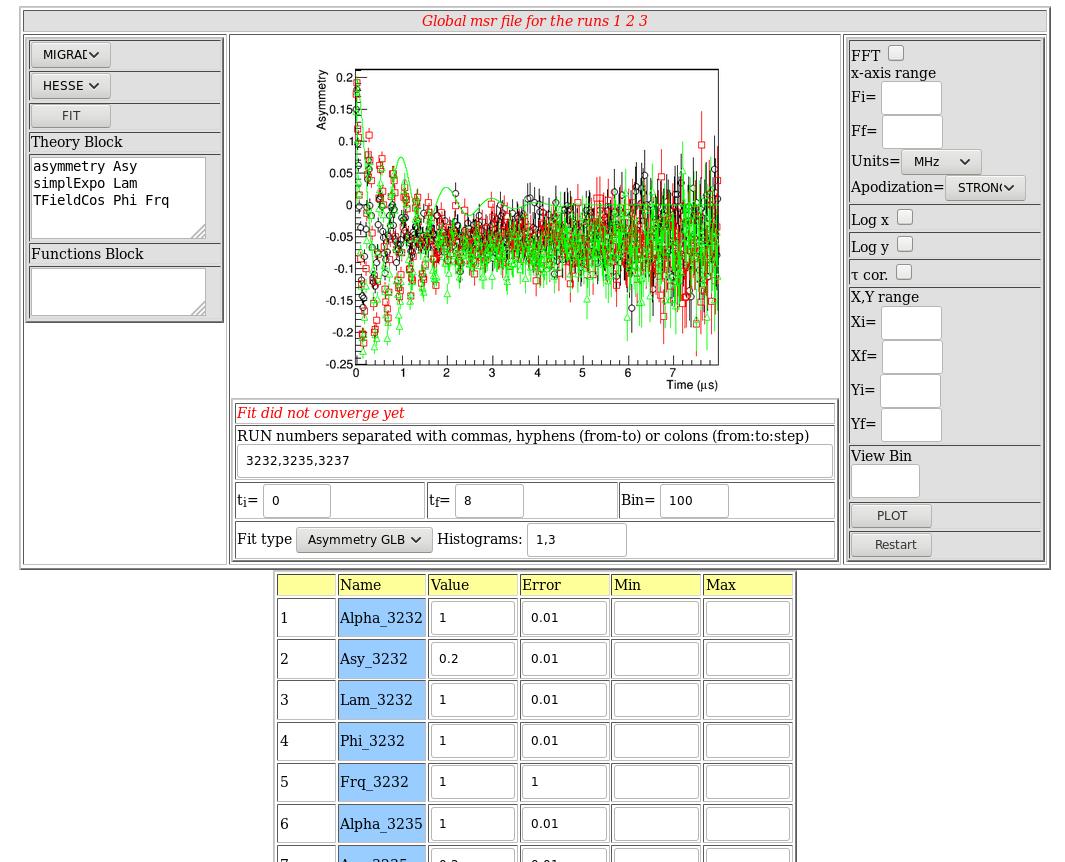
At this stage you can also change or fix the value of fit parameters. The musrfit.cgi script typically starts with reasonable default value for various parameters which will usually be a good enough guess for simple fits. However, care should be taken when performing a more complex fit, since a bad starting guess may lead to the fit not converging at all. For each fit parameter you can give an initial value, error, minimum and maximum values:
- the value determines the initial guess
- the error determines the initial step in the fitting procedure. If the error is set to zero “0”, then musrfit will assume that the corresponding fit parameter is fixed at the given value
- the minimum and maximum values provide the boundaries that will be imposed on the corresponding fit parameter.
Once all parameters have been adjusted (or if you are happy with the defaults) click on “PLOT” to plot without running the minimization of “FIT” to run the fitting and minimization before plotting the result.
On this page you may also change many of the fields that you set in previous stages on the fit. Just below the figure you will be able to change the run numbers that you are fitting, add additional runs to the fit or remove runs from the fit. You may even change the order or number of histograms that were used from the fit in the “Histograms” field. You can also change the fitting time range by changing “ti” and “tf”.
On the right hand side you will be able to change various aspects of the plot. These will only change the displayed figure, but will not change the actual fit itself. You can inspect the FFT of the plot.
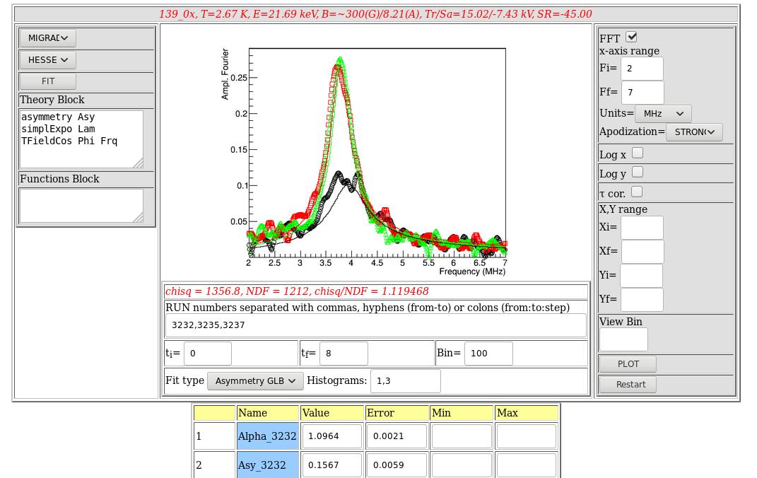
You may toggle between log and linear x or y scales using the appropriate check box. “t cor.” can be used to correct for the muon lifetime in single histogram fits. The “x,y range” can be used to change the x and y scales.
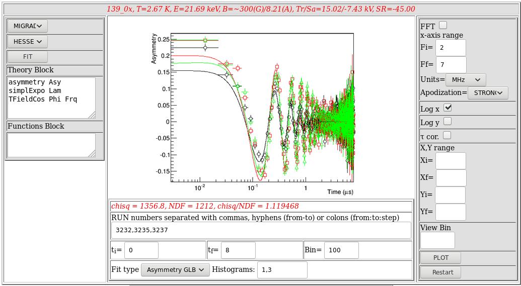
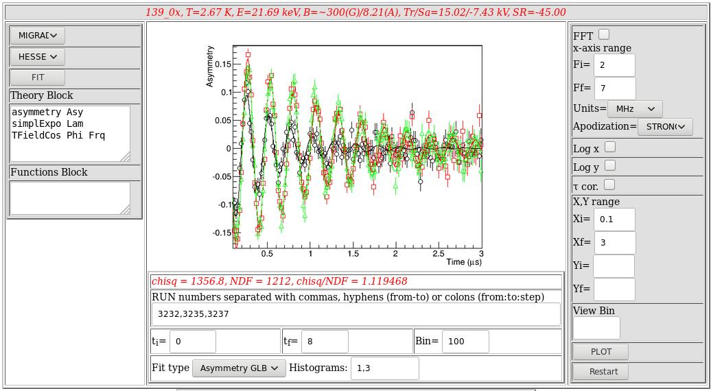
“View Bin” can be used to re-plot the same fit using a different binning factor from that used for the fit, which can be sometimes very useful to more clearly inspect the quality of the fits. Any change in these fields will not take effect until you press the “PLOT” button (or the “FIT” button on the right hand side, see below)
On the left hand side you will be able to control the minimization for the fit. For the minimization you can choose between “MIGRAD”, “MINIMIZE” or “SIMPLEX” which indicate different minimization routines used by minuit. For the error calculation you can choose either “HESSE” or “MINOS”. The first is fast but less accurate than the latter. Once these are selected you can press on the “FIT” button which will run the requested minimization and error estimate. The results of the fit are displayed in the same page and the values and errors in the fit parameters are updated. This stage can take some minutes so be patient and avoid using this script for fitting many (more than 20) runs and/or for very complex fits.
An extremely useful aspect of this script is that all fit results can be downloaded and used immediately to generate quick plots of the parameters. At the bottom of the page you will find links to five different files:

- FileName.msr – is the musrfit input file which can be downloaded, edited and used as a starting input file for more complex fits or as a template for different fits.
- FileName.dat.gz – is an archive that includes ASCII files which contain the data points with error bars as well as the fit curves. This can be easily used to generate plots of the displayed figure in your favorite plotting software.
- FileName_par.dat – is and ASCII file which contains the values of the fit parameters in a table format. This can be easily used to plot the dependencies of the various fit parameters on temperature, field etc.
- FileName.out and debug.txt – Are files for debugging information. If you have a problem, it would be best if you send usthese files by email.
