Parameters and parameter plots
The Parameters tab shows the numerical model: one row per fitted parameter, per data set, with starting values, steps, and limits. Fitting feeds the measured values back, and the same table drives the interactive parameter plots.
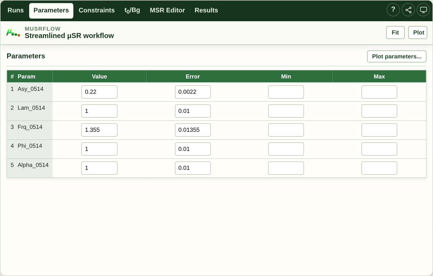
Example parameter table before fitting, for the same run and model as Getting started. These are initial values, not measured results; the Error column contains starting steps at this stage.
The parameter table
The table is rebuilt automatically whenever the model changes (a new component, a new run, a constraint). Rows are keyed to the model:
Single-run fit: one row per parameter of the selected model.
Multi-run fit: a row per parameter per data set, each named by its run (for example
Lam_2255), plus the parameters you choose to share.
Rows follow the physical role of each parameter: the initial asymmetry first,
then the relaxation/lineshape parameters, then the precession frequency, then
the phase, then the asymmetry alphas and group ratios, and finally the
detector normalization/background parameters. This ordering is what ends up in
the generated FITPARAMETER block and therefore in the *_par.dat columns
from msr2data. A parameter introduced through a constraint (for example
Bfield = gamma_mu * Frq) is placed with the built-in parameter it is linked
to; when it is linked to several parameters it takes the highest-priority
(lowest) rank among them. An order imported from an existing MSR file always
overrides this physical sequence.
For each parameter the columns are the starting value, the step, and the lower/upper limits. Edit any of them directly. Run-scoped parameters are matched to their data set by the run suffix, so a per-run starting value only affects that run. The values in this table are the starting values used for the next fit; after a fit they are replaced by the fitted results, and the fit uncertainties are available in the parameter plots as error bars.
Selecting parameters for plotting
Click a parameter name to select or deselect it for plotting:
Click – toggle that single parameter.
Ctrl / Cmd-click – add an individual parameter without changing the rest of the selection.
Shift-click – select a contiguous range of parameters.
Long-press (touch) – on mobile/tablet, long-press a parameter name to add or remove it from the selection without clearing others (multi-select).
The selection state is shown in the row. Then use the Plot parameters… button at the top of the parameter table to open the plot window. If the parameter table is not yet populated (no fit run yet and no file loaded), the plot can still build the parameter data inline from the table – the button stays enabled whenever the table is built.
The Choose X axis dialog
The dialog lists the parameter data columns and asks which one to use as the common X axis. Each selected parameter becomes a Y series.
The dialog also offers the Layout of the plot window:
Auto – one parameter per panel. Up to three parameters share a single column; beyond that the panels grow toward a square grid (two parameters in two columns, three in three, and four or more arranged as the closest square grid).
Single row – all parameters side by side in one row.
Single column – all parameters stacked in one column.
The layout choice is remembered for the next plot. The window opens with the chosen arrangement, and the Plot options panel lets you re-arrange the panels afterwards.
The parameter-plot window
The window shows one panel per data set / parameter as arranged by the layout choice. Panels share the chosen X axis. The toolbar holds:
Refresh – reread the current parameter-data file and redraw every visible panel. Use this after a new fit to update the numbers.
Data… – change the data set loaded in the active panel.
Add data set… – choose one or more parameter-data files and overlay them onto every panel at once. Each file keeps one colour from the Palette, and every panel plots the parameters it already shows for each newly added file, so a scan can be compared against the current one across the whole window with a distinct colour. The Y-axis label stays on the active panel’s parameter rather than reverting to a generic label. Adding files this way is the same overlay mechanism as Overlay data sets in Plot options; the toolbar shortcut just applies the additions to all panels instead of the active one.
Overlaid curves get a smart legend label that says which physical state
each scan represents instead of only a file name. The label is derived from
the data set’s own scan variable and its constant coordinate: an energy scan
(dataE varying) is tagged with its fixed temperature ((T = 300 K)), a
temperature scan with its fixed energy for LE-µSR ((E = 12 keV)) or with
its field for bulk µSR ((B = 100 G)), and a field scan with its fixed
temperature. When no fixed coordinate is present the plain file label is used.
You can also rename a legend entry directly in the plot; a Refresh then keeps
your name instead of rebuilding the default.
Plot options – expand the layout, X, parameter, style, and displayed series controls for the active panel.
Plot options
Layout – the concrete panel grid (for example
1 x 1…3 x 3and larger grids as the panel count needs). Changing it adds or hides panels; new panels start empty and clone the sync settings of the current panel.Panel indicator – which panel is active (
Panel 1/3). Click a panel to activate it before changing its panel-specific settings.Data set – the data source shown in the active panel.
X – the X column for the active panel.
Parameter – add a Y parameter to the active panel. Serial chips underneath list the current Y series; click the
xon a chip to remove that series.Style –
Scatter,Lines + markers, orLines.Palette – the base colour palette (
Default,Bold,Pastel,Monochrome) used to assign each overlaid data set its default colour. Changing it restyles every panel.X title / Y title – override the automatic axis label of the active panel; leave empty to keep the automatic label.
Remembered plot configurations
The full window state is remembered per data source: the panel arrangement, the X column, the template, the palette, the per-series styles (including the error-bar caps setting), and the overlay files. A configuration is keyed by the data source and the parameter set it plots, so each parameter selection has its own remembered configuration.
Restoring a configuration is always an explicit choice, never something that happens behind your back:
The Choose X axis dialog appears every time you plot parameters.
If a remembered configuration matches the parameters you selected (the same set, in any order), a Configuration dropdown appears in the dialog. The most recent matching configuration is preselected; the dialog shows exactly what will be restored, and you press Plot to confirm.
Choosing From scratch in the dropdown (or having no matching configuration) starts a normal new window from the X axis and layout choices on the dialog.
Matching is exact: a saved configuration for three parameters never shows up for a one-parameter request, even if that one parameter is part of the three.
State is keyed by the data source, so
scanA_par.datkeeps its own styles and layout while other files (and their overlay sets) remember theirs independently.Up to eight data sources are remembered; adding a new one forgets the oldest. Each source keeps at most one configuration per parameter set (the newest wins) and a handful of parameter sets in total.
Forget plot configuration in Plot options clears the remembered state for the data source shown in the active panel, so the Choose X axis dialog offers no configuration next time.
The remembered configuration of the current data source is carried in configuration share links, so a colleague restoring your link gets the same plot window – see Configuration sharing. When a real fit produced the parameter table, the table itself is embedded in the link (inline text) and a web restoration renders the identical plot immediately, without needing a local or server-side fit.
Uploaded files keep only their identity, not their contents: if the original file cannot be read again (for example it was deleted), the restored plot degrades gracefully and the dialog is offered instead.
Overlay data sets (multiple files in one panel)
Panels can plot several *.dat files at once so scans can be compared on
one set of axes. Open Plot options and use Overlay data sets > Add
file… to choose extra parameter-data files (on the desktop this is a
native multi-select dialog; on the web it is the browser’s multi-file
picker). Each file becomes a row with a checkbox:
checked rows are drawn on top of the panel’s main data set;
the colour swatch shows the default trace colour for that file, assigned from the Palette;
files are identified by their resolved path or blob identity, so picking the same file twice keeps one entry – and one user-adjusted style;
the X axis is aligned across files by column name – a file that does not contain the panel’s X column is skipped and named in a striped note under the panel;
in overlay mode each file’s traces share its colour, and legend entries are prefixed with the file name (
scanB_par.dat: λ₁).
Growing the layout clones the active panel, so expanding a 1 x 1 grid to
2 x 1 carries the overlay files into the new panel. Unchecking a row
removes that file from the active panel only; the file stays available in the
list for other panels.
Worked example: energy scan at two temperatures
See LEM single-histogram example for the complete illustrated walkthrough and reproducible results. It uses new single-histogram fits of LEM 2025 runs 1014-1027 (blue, 3.8 K) and 1033-1045 (red, 10 K), not the older asymmetry-fit reference tables.
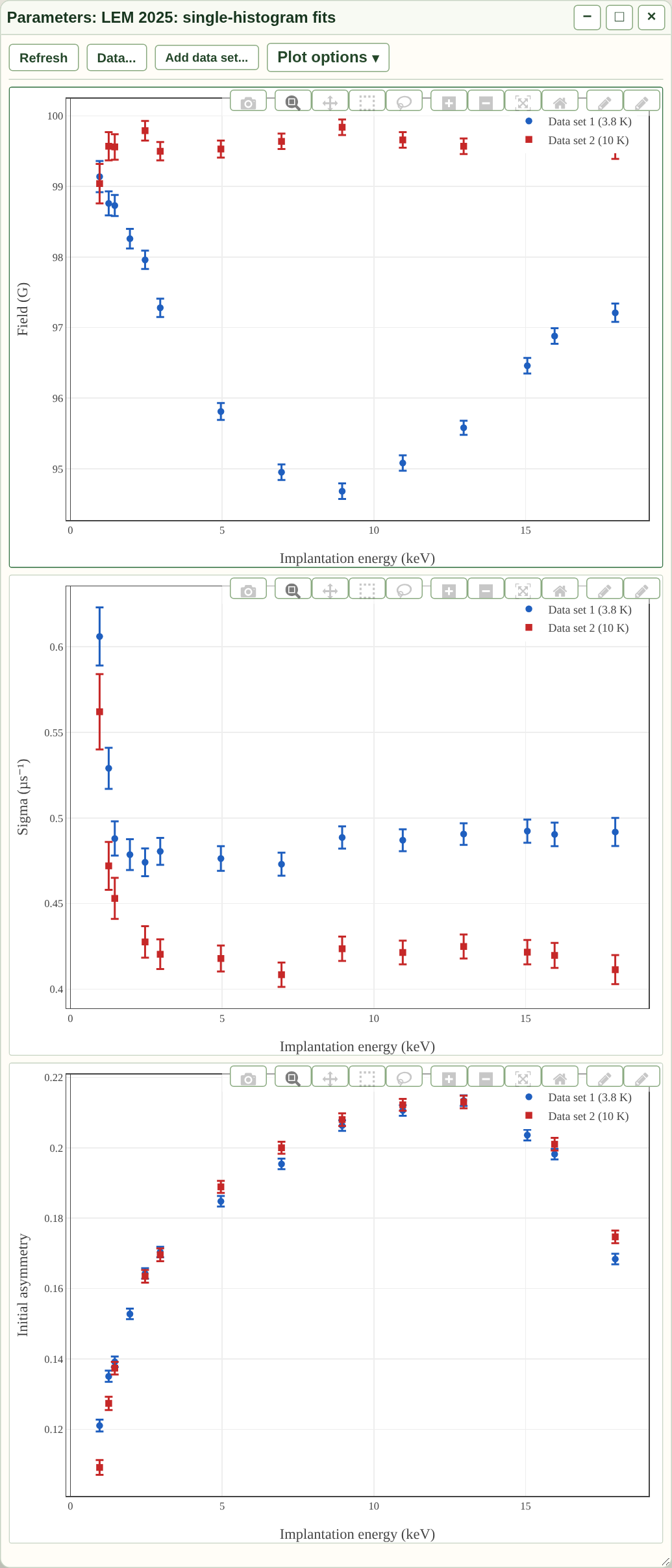
Three vertically stacked panels from the application, using the newly
fitted single-histogram tables. Both data sets are overlaid in each panel.
The example chapter explains the model, histogram grouping, uncertainties
and limitations; results are in
docs/examples/lem2025-singlehist-energy-scan.
Editing trace styles
Click any marker directly in a plot panel to open a small style editor near the pointer:
This trace / This data set – whether the change applies to the clicked (file, parameter) series only, or to every trace of that data set (all panels showing it). Choosing This data set unifies the whole file and clears any per-panel trace styling left behind, so those panels no longer shadow the new style.
colour swatches, marker symbol, size, and opacity;
Error-bar caps – error bars are plain vertical lines unless the checkbox is ticked, which draws the cross-bars at both ends;
Apply – commit the staged choices and redraw the affected panels; Close hides the editor, and ESC (or
Q) dismisses it;Reset – restore the file’s default colouring for that scope.
Trace-level edits are keyed by (data set, panel, parameter), so they survive
panel re-layouts but never leak onto other panels. Data-set-level edits are
shared: recolour scanA_par.dat once, and every panel that shows it
updates. Esc (or Q) closes the editor; the title bar is a drag
handle so the panel can be repositioned within the parameter-plot window.
Template and series presets
The Template dropdown applies a predefined multi-panel arrangement that
maps recognised parameter names to roles. For example the tf-scan
template lays out three panels – amplitude, damping, and frequency – above
one another. Parameters that cannot be matched to the data are omitted
rather than guessed; unmatched panels stay empty.
Keyboard shortcuts
With a panel focused (and not while typing in a field), the shortcut keys are:
u– reset the active panel to its automatic X and Y ranges.QorEsc– close the plot window.
The plotly mode bar at the top-right of each panel provides zoom, pan, box select, and download, and a custom button toggles each axis between linear and logarithmic. Trace colours are assigned automatically per series – clicking a marker opens the style editor described above to change them.