Runs and fitting
The Runs tab holds everything that selects and describes the data: the run list, the fit range, the fit model, the fit options, and the view settings used for Plot, FFT, and RRF.
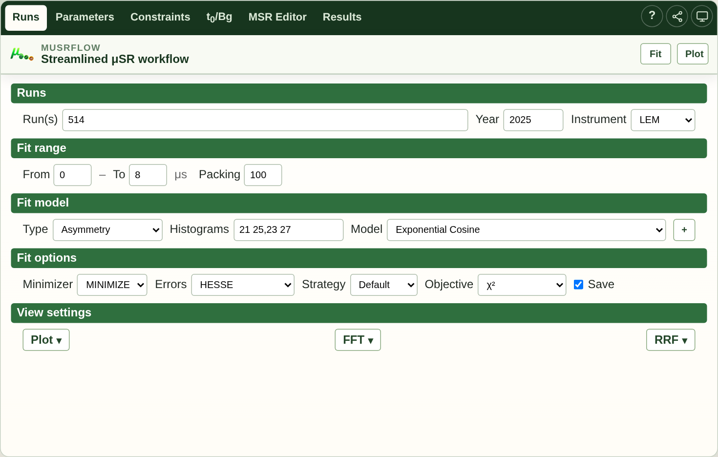
The Runs tab combines data selection and model preparation. Fit and Plot remain available while working in the other tabs.
Run selection
- Run(s)
One or more runs, separated by commas. A dash selects a contiguous range and a colon-with-step
from:to:stepproduces a regular sequence, for example520:540:2.Each comma- or range-separated data set is fit independently and merged into one fit document, so
514, 516, 520-525prepares eight data sets.A
+between runs adds the run to the previous data set via the MSRADDRUNdirective rather than starting a new data set.514+515is a single data set composed of two runs.Examples:
514– one run.514, 520-525– seven data sets: 514 and each of 520..525.514+515, 520:540:2– one ADDRUN data set and a stepped range.
- Year
The data-taking year. The year range starts at 1998 and cannot exceed the current year.
- Instrument
The spectrometer. The exact choice (for example LTF, FLAME, LEM, GPS, GPD, Dolly, VMS, HAL) depends on the data tree your installation exposes.
The path shown in the resolution warning below the row confirms that the chosen runs resolve to real data files; a successful resolution is silent.
- Mixed sources
Choose Mixed when one fit must combine data from different years, instruments, or explicit data-file paths. Mixed input has its own syntax and execution route; see Mixed run sources for the complete procedure and current limitations.
Fit range
From / To – the time window in microseconds that is actually fit (default
0to8).Packing – the time-binning factor used for the fit (default
100).
Fit model
- Type
The fit type. Asymmetry is the normal choice for a summed forward plus backward count rate. Single hist fits a single histogram. The legacy Asymmetry (Legacy) variant is kept for old MSR files that used the classic syntax but is not offered for new documents.
- Histograms
The detector histograms, or a packed detector name, that make up the asymmetry signal.
An Asymmetry fit normally takes one forward,backward pair (for example
21 25). Several groups of one physical run can be fit at the same time by entering slash-separated forward,backward pairs, for example1,2/3,4for two groups (detectors 1 and 2 form the first group, 3 and 4 the second). Each group becomes its own RUN block with its ownalphaand phase, and the groups scale a shared free amplitude by individual ratios (the first group keeps the fixed identity factor). The parameter table carries a per-groupAlpha,Phi, and ratio; the physical model parameters stay shared. Multi-component models and per-run pairs of a multi-run (global) fit are not eligible for the multi-group route.- Components
The theory model is a sum of components. The first component is labelled Model and is required; further components are added with
+and can be removed with thexon their row. Each component has its own parameter set, shown in the Parameters tab.The component list is grouped by physics:
Relaxation –
Asymmetry,Exponential,Gaussian,Stretch.Static KT –
SLKT,SGKT,LGKT,STRKT,GBGZF.Oscillating –
ExponentialCos,GaussianCos,StretchCos,AbragamCos,GBGCos,ExponentialBessel,GaussianBessel.KT x relaxation – combined Kubo-Toyabe and relaxation functions, e.g.
LLFExp,GLFExp,LGKTExp,GBGExp,STRKTExpand their spin-flip variantsLLFSExp,GLFSExp,LGKTSExp,GBGSExp,STRKTSExp.Dynamic KT –
LDKTLF,GDKTLF.
Changing a component rebuilds the parameter table and the constraint preview so their contents follow the new model.
Fit options
Minimizer – Minuit2 strategy variant used by the fit:
MINIMIZE(default),MIGRAD, orSIMPLEX.Errors – the error calculation run after the minimisation:
HESSE(default),MINOS,HESSE + MINOS, orNone.Strategy – Minuit2 strategy
0,1,2, or Default (leave unspecified).Objective –
χ²(default) or Max likelihood.Save – write the detailed Minuit2 output including covariance information (on by default).
Series fit actions
When two or more independent data sets are fit together without shared parameters, the fit follows the independent-series route and the Fit options row gains a per-run action chip for every data set. This is how a multi-run series is (re)fitted efficiently without re-fitting runs that have not changed.
Clicking a chip cycles through three actions:
reuse – keep the existing fit result for that run.
refit – rebuild the MSR from the live GUI parameters and fit again.
skip – leave the run untouched.
The All dropdown applies one action to every chip at once (Reuse all / Refit all / Skip all), which is the convenient way to set a uniform policy and then override single runs by clicking their chip.
A series where every run is skipped reports Nothing to fit. Sharing any parameter (the Shared column in the parameter table) disables this route and the chips disappear; see Parameters and parameter plots. The parameter plot is unaffected and still works.
Per-run statistics
For an independent-series fit the status-bar statistic button summarises the
series – either Series did not converge (some runs failed to converge) or
a worst/best aggregate such as χ²/NDF worst 1.24 / best 1.01 · 5 runs.
Clicking the button opens a per-run statistics table that lists every data set
in run order with:
the run identifier;
the action that produced it (reuse, refit, or skip);
the run’s statistic text (χ²/NDF or max likelihood/NDF, or
Fit did not converge);the converged state;
the fitted file the value came from.
Reused or skipped runs show the values read from the MSRs already used for plotting. Rows are highlighted for contrast: runs whose value is more than twice the series median stand out as outliers (the spread a worst/best summary might hide), failed runs are marked as not converged, and reused/skipped rows that still carry the on-disk value are visually distinct from freshly fitted ones.
View settings
Plot, FFT, and RRF are one-row disclosure buttons; each expands its settings inline, and only one group is open at a time. The dots next to the buttons mark a group whose settings differ from the defaults.
- Plot
Time range – independent start and end of the displayed time axis; leaving a field empty selects automatic limits.
Y range – independent displayed Y limits; empty means automatic.
View packing – histogram packaging for the view; empty means automatic.
Log X / Log Y – switch the respective displayed axis to a logarithmic scale.
Lifetime correction – apply the lifetime correction to the displayed spectra (on by default).
- FFT
The Fourier-transform display settings:
Type –
Power,Real,Imaginary,Real & imaginary, orPhase.Apodization –
Strong,Medium,Weak, orNone.Phase – the phase value or a musrfit phase expression, for example
8.5,par7,par(7,5,16),parR(...).DC correct – remove the time-domain DC offset before the transform.
Range – the frequency window used for the transform; empty means automatic.
Units –
MHz,Gauss(default),Tesla, orMc/s.Power – the
powerrecord for the FFT (default12).Phase correction – automatic phase correction
Off, over the FFT range, or over a Custom range you type below.
- RRF
Rotating-reference-frame display settings. They are strictly opt-in: opening the settings does not change the generated plot block.
Enable – add rotating-reference-frame directives to the PLOT block.
Frequency – the reference frequency, with units
MHz,kHz,Mc/s,Gauss(default variety shown as Gauss), orTesla.Packing – the packing for the RRF view (required when enabled).
Phase – optional phase in degrees, or a parameter reference such as
par4.
Fit and Plot
The two toolbar actions work on the current window state:
Fit – validate the run selection, prepare the MSR document from the GUI, and run
musrfit. The fitted values flow back into the parameter table and the results.Plot – validate the run selection, prepare the same MSR document, and run
musrviewto display the spectra. On the web the resulting ROOT canvas is drawn inside the page window with JSROOT; on the desktopmusrviewopens its own native window.
While either action runs, the status bar shows progress and the Results tab accumulates the command log. Plot-compatible values are cached so a plot does not lose the numerical fit quality already returned by a previous fit.
On the desktop, a local Fit uses every available CPU core by default. Set
musrfit threads in Preferences to cap the OpenMP thread count
(musrfit -u) when a machine is shared or a fit would otherwise saturate
the login node; leaving it blank keeps the all-cores behaviour. The web
edition always fits on the server and ignores the setting.
If the MSR editor owns the document (a hand-edited MSR is authoritative), the editor block is used for Fit and Plot as-is and GUI changes do not silently replace it – see MSR editor.