Tutorial 1: File format and Templates

In this tutorial we are going to modify an existing template file to analyse a weak transverse field alpha calibration measurement on silver, which was measured on FLAME as run number 804 in 2024.

Prerequisites

This Tutorial assumes you have a working musrfit installation. Installation instruction and a full documentation of musrfit can be found at https://lmu.pages.psi.ch/musrfit-docu/ .

The musrfit program contains terminal executables for most available functions. However, in this tutorial we will only use the graphical user interface musredit.

Opening a template file

In almost all use cases, you don’t write a musrfit file from scratch, but start by adapting an existing template file to your needs. Let’s assume you have been given a musrfit file 1703_Ag.msr with a measurement on silver in zero field, and you want to modify it to a weak transverse field measurement. Note that we start with a very unsuitable template on purpose, so we will have to adjust quite a lot of things until we arrive at a good fit. In most cases, you will have a more suitable template to start with.

Open musredit by double-clicking on the app, or by running musredit & in a terminal.
Open the template file in tutorials/1.0/template/1703_Ag.msr . You can either use File -> Open… in the top menu bar, click the file open button , or use the Ctrl+o keyboard shortcut.

File structure overview

If you look at the file, you will notice that it is structured into different blocks by using keywords. Each block has a specific function and we are going to look at these in the following tutorials in detail.

Title: The first line of the msr file is the title line, in which any information can be placed.
FITPARAMETER: The FITPARAMETER block lists all fit parameters and their boundaries.
THEORY: The THEORY block is used to define the fit function.
FUNCTIONS: The FUNCTIONS block is optional and can be used to define auxiliary functions.
GLOBAL: The GLOBAL block is optional and can be used to specify information that is the same for every run entry of the RUN block.
RUN: The RUN block is used to describe the data of a particular measurement that should be fitted.
COMMANDS: The COMMANDS block is used to specify the sequence of actions that should be performed when fitting the file.
FOURIER: The FOURIER block describes how the Fourier transform of the data should be calculated and plotted.
PLOT: The PLOT block defines how to plot the spectra.
STATISTIC: The STATISTIC block summarises information from the last fitting. It’s content should not be edited.

Tip

Whenever you are in doubt about the available keywords, their function or the exact syntax to use in any of these blocks, check the corresponding section of the user manual: https://lmu.pages.psi.ch/musrfit-docu/user-manual.html#description-of-the-msr-file-format

Verifying file integrity

The easiest way to check the syntax of a musrfit file to see if it wil fit/plot correctly is to try to calculate chi-squared. We can try this now:

Click on the calculate chi-squared button.

For your template file, you will get an error. Obviously there is something wrong with it:

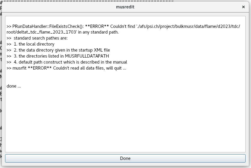
This error message means that the syntax of your musrfit file is probably alright, but that the previous raw data deltat_tdc_flame_2023_1703.root could not be found. This is not very surprising, since you are missing the corresponding /afs/ mount. We will anyway need to change that to our wTF measurement, which you can find in data/deltat_tdc_flame_2024_0804.root . So let’s try to do that now.

Changing the raw data file

In order to avoid overwriting the template file, we will save it under a new name.

In the top menu bar select File -> Save As… and rename the current musrfit file to 804_wTF.msr.

Important

The filenames of musrfit files should always start with the run number. The reason for that will become clear later, when we look at parameter export, global fits and chain fits. Adding other useful information (here we have added _wTF) is optional. Moreover, make sure to always specify the file extension .msr .

As mentioned before, the data is described in the RUN block. So this is where we need to change the file. In particular the line we want to change is:

RUN /afs/psi.ch/project/bulkmusr/data/flame/d2023/tdc/root/deltat_tdc_flame_2023_1703 PIM3 PSI MUSR-ROOT   (name beamline institute data-file-format)

To point musrfit at our new datafile, we can specify both an absolute or a relative path. So if your file is saved in the same folder as the template file, the following substitution should work:

RUN ../../../data/deltat_tdc_flame_2024_0804 PIM3 PSI MUSR-ROOT   (name beamline institute data-file-format)

However, this might cause you more work down the line whenever you change something about your folder structure. So the more well defined way is to adjust your default search paths:

Click on the Preferences button, then on Change Default Search Pahts with Add select the data folder .

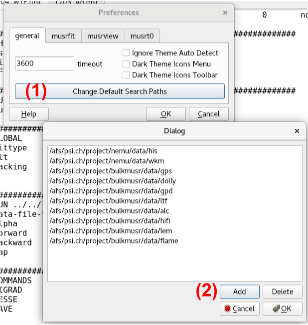
Now you can simplify the RUN line to:

RUN deltat_tdc_flame_2024_0804 PIM3 PSI MUSR-ROOT   (name beamline institute data-file-format)

Press the button, to see if this worked. If successful, you should now only get warnings, but no errors. Moreover, the resulting chi-squared divided by the number of degrees of freedom is calculated to be chisq/NDF = 308.9. Therefore, while the file is technically correct, the fit is terrible.

Adjusting T0, data and background

It is usually a good idea to take care of any warnings in chi-squared before trying to optimise how to correctly fit the data. The reason we received warnings above is that we are missing the t0, data and background keywords in the RUN block, and did not do a t0-calibration. Therefore, some default values are assumed at the moment, which may or may not be correct.

Lets add the missing keywords with some reasonable defaults to the RUN block:

t0              1600.0  1600.0
data            1620    102401  1620    102401
background      160     900     160     900

Now the warnings in chi-squared should be gone. However, we potentially made the situation worse, because the default might have been better than our guess.
To determine the correct values, we need to do a t0 calibration. Start it by clicking the T0 button. This opens an interactive window plotting the raw histogram of the forward detector in the first RUN block:

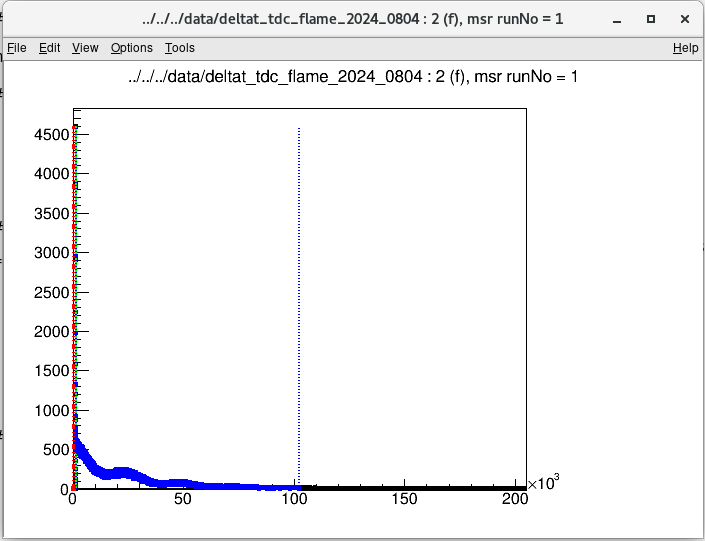
The green line represents time zero, the start of the spectrum. The blue lines show the range of valid data range and the (optional) red lines give the limits of the region from which the uncorrelated background is estimated.

The window is interactive, and you can use the following keyboard shortcuts to adjust the parameters:

`Shift`+`T`	Automatically move the green t0 line to the bin containing the maximum number of counts.
`t`	Move the green t0 line to the current cursor position.
`z`	Zoom to the region around t0.
`u`	Undo the zoom of the spectrum.
`b`	Set the lower limit of the red background range to the current cursor position.
`Shift`+`B`	Set the upper limit of the red background range to the current cursor position.
`d`	Set the lower limit of the blue data range to the current cursor position.
`Shift`+`D`	Set the upper limit of the blue data range to the current cursor position.
`q`	Save values and continue with the next histogram.

Tip

If the window does not react to a keyboard shortcut, select it by clicking on it, and try again.

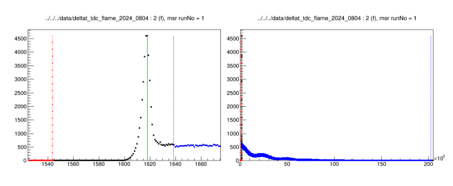
For both forward and backward histogram, set Shift+D to the end of the spectrum, use Shift+T to find the prompt peak, and set d to shortly after the prompt peak. You might find this easier by pressing z to zoom in on the prompt peak. You can also move Shift+B to higher values, but keep it far away from the prompt peak. Confirm with q. You will then need to repeat the procedure for the second detector.
Check the RUN block and ensure the values are updated. They should now look something like the following. Note that the t0 values are most important; anything close to the values below is ok for the other parameters.
```
t0              1618.0  1628.0
data            1639    202527  1649    202160
background      160     1544    160     1544
```

Plotting spectra and fitting

Plot the spectrum by pressing the view button.

Looking at the spectrum, the following problems are immediately obvious:

The binning on the plot is too high.
The solid fitted line is not describing the spectrum at all.

We can change settings for plotting such as binning in the PLOT block of the musrfit file. Reduce the binning by changing the value for view_packing to 1000. We can also relax the y-axis limit on the plot_range, to ensure all the data is displayed:
```
###############################################################
PLOT 2   (asymmetry plot)
runs        1
plot_range 0.3 10 -0.5 0.3
view_packing 1000
###############################################################
```

Once you have updated these parameters, you need to press the view musrview button again to get a new plot.

Warning

The binning for plotting and the binning for fitting are two independent numbers. If you want to change the binning used in fitting you need to change the value of packing, which is specified either in the GLOBAL block or in the RUN block.

The fitted line is still completely wrong, but we haven’t tried fitting yet. Do so by clicking fit button .

This should have improved chi-squared significantly, but we are still far off from chisq/NDF ~ 1 which would indicate a good fit. If you plot the data again, you will notice that the result of the fitting is a constant line at -0.18 without any oscillation. In addition, if you have a look at the resulting values in the FITPARAMETER block, you will see some completely un-physical values. So just blindly fitting will not work because our template contains the wrong fit function.
Undo the most recent fitting, by clicking the Swap Msr <-> Mlog button to recover the previous parameter values.

Changing the fit function

The fit function is defined in the THEORY block. Here you can combine a set of predefined fitting functions, see https://lmu.pages.psi.ch/musrfit-docu/user-manual.html#the-theory-block .

Important

By default, subsequent lines are implicitly multiplied. If you want to add them instead separate them with a line containing a + sign.

At the moment our fitting function is:

###############################################################
THEORY
asymmetry      2
statGssKt      3          (rate)

The numbers indicate the corresponding parameters in the FITPARAMETER block. Therefore, we are fitting a Kubo-Toyabe function:

\(A_0 \left(\frac{1}{3} + \frac{2}{3} \left[ 1 - (\sigma t)^2\right] \exp\left[-\frac{1}{2} (\sigma t)^2\right]\right).\)

Instead, we would like to fit a Gaussian-damped oscillation:

\(A_0 e^{-\frac{1}{2} (\sigma t)^2} \cos\left(2\pi\nu t + \frac{\pi \varphi}{180}\right).\)

Looking at the manual, we see that we can combine the functions simpleGss and TFieldCos to achieve this parametrisation.

Change the THEORY block accordingly:

###############################################################
THEORY
asymmetry      2
simpleGss      3          (rate)
TFieldCos      4  5      (phase frequency)

Tip

Each function has an abbreviation, so you can also write the following short version. The first time you fit, this will be expanded into what we wrote above:

THEORY
a 2
sg 3
tf 4 5

If you now press chi-squared musrchisq , you will immediately get an error. The reason is that we just introduced new parameters (number 4 and 5) for phase and frequency, without specifying them in the parameter block.

Adding parameter and limits

Each parameter in the FITPARAMETER block has a number, a name, a step (which is a guess for the standard deviation), and a posError (which is an output parameter that is used if you specify the MINOS error estimation in the command block to provide asymmetric error intervals). Optionally, each parameter may also have boundaries.

Important

The parameters must be numbered consecutively starting at 1 and the names must be unique.

To add the missing parameter append the following two lines to the FITPARAMETER block:

4 Phi         0         1           none
5 Frequency   0.3       1           none

Don’t worry about the indentation or white spaces, these will automatically fix themselves when you fit the file.

Fit the data and plot it.

You can see that we are getting closer, but still the oscillation is not fully captured, and it is not centred around zero. This is the case because the alpha parameter was fixed by setting its step to 0. However, our current sample has a different alpha than the one used in the template.

Allow fitting of alpha by setting a non-zero step:

1 alpha       0.80606   0.1           none

The value you pick for the step tells musrfit how big the first step in the optimisation should be. You should pick a value that is neither too big or too small.

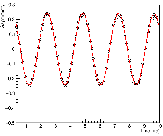
Fit and plot again. Now the fitting should be a lot better with a more reasonable chisq/NDF = 1.012

Tip

If you only plot a single spectrum, you can highlight the fitting function by clicking on the display window, and then pressing the t key.

Note that with this parameterisation the values of asymmetry, sigma and frequency could all fit to a negative value. There are two ways to avoid this.

If you notice that this happened, you can in most cases just change the sign of the starting value and fit again.
We can add a lower limit of 0 for the parameter. Let’s try this now:

Change the parameter block as follows and then fit musrfit again:

FITPARAMETER
###############################################################
#      No Name        Value     Step        posError  [Lower_Boundary Upper_Boundary]
        1 alpha       1.16105   0.00056     none
        2 Asymmetry   0.24501   0.00036     none        0       none
        3 Sigma       0.0244    0.0037      none        0       none
        4 Phi         -0.17     0.12        none
        5 Frequency   0.41481   0.00011     none        0       none

Now all parameters should be positive.

Using functions

We have now correctly fitted the spectrum to an oscillation frequency. However, in many cases, we would like to instead parametrise it as a function of the local magnetic field. We can do this by adding an auxiliary function.

Rename Parameter 5 to Field:

5 Field   0.41481   0.00011     none        0       none

Uncomment the FUNCTIONS block and define a function (fun1) which is the muon gyromagnetic ratio multiplied by parameter 5:
```
###############################################################
FUNCTIONS
fun1 = gamma_mu * par5
```

Important

Functions must be named funN with N being the number, starting at 1.

In the theory block, specify that fun1 should be used as frequency instead of parameter 5 :
```
TFieldCos      4     fun1      (phase frequency)
```
Fit again, and you should see that now, you have a field of about 30.6 G in parameter 5. If you don’t get a good fit, you might need to change the initial field to a better guess before starting. Remember you can undo the last fit with the Swap Msr <-> Mlog button .

This concludes the first tutorial. If you get stuck, you find an example of how your file might now look like in tutorials/1.0/solution/804_wTF.msr .