Tutorial 3: ZF and chain fits

In this tutorial, we will learn how to do a fast analysis of a large dataset, a procedure particularly suitable for initial data analysis during an ongoing experiment. In the data folder, you find a dataset with zero-field measurements on in polycrystalline MnP, measured with the GPS spectrometer and published by R. Khasanov, et al., in Phys. Rev. B 93, 180509(R), (2016) . You can use the data under CC BY-SA 4.0 with permission from the authors.

Determine geometric parameters

Whenever we analyse a zero field spectrum, we need to have an independent calibration of the geometric alpha (and beta) parameters with a weak transverse field measurement. Otherwise we might misinterpret our data, for example missing if our spectrum has a non-zero baseline in ZF. For the current example this is particularly relevant, since in for a polycrystal in ZF we expect a powder average where 2/3 of the initial asymmetry oscillates, whereas 1/3 can only relax dynamically.

You can find a room temperature alpha calibration for this sample located in data/deltat_tdc_gps_0222.bin . The files in this tutorial were written in a legacy .bin file format. Simply specify this as a different data-file-format in the run block.

RUN ../../../deltat_tdc_gps_0222 PIM3 PSI PSI-BIN   (name beamline institute data-file-format)

There is a wTF template in tutorials/3.0/template/69_wTF_template.msr. Note that in this file we also simultaneously analyse the up-down detectors, as well as the forward-backward pairs we have looked at before.

• Redirect the template at your measured data file.

• Check t0. (In the psi-bin format this actually matters even more.)

• Fit and determine alpha and beta for the up/down detectors.

Hint

Obviously, all of this is a repetition of what we did previously. If you want to skip it, you can continue by assuming that both values are equal to 1.

Chain-Fitting

• Open file tutorials/3.0/template/232_ZF.msr.

• Paste and fix the previously determined alpha and beta values for the up-down detectors.

• Fit and have a look at the spectrum.

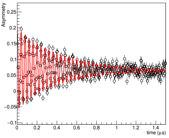
What you have here is a fully analysed spectrum of MnP in zero field at 250 K in its ferromagnetic phase. It exhibits a single oscillating frequency and a tail. However, a experiment seldom consists of a single measurement. What you have in runs 232-260 is a temperature scan measured upon warming up to 300K. If we wrote and fitted .msr files for all of these, then copied the resulting parameters to a table, we woudl still be here tomorrow. Instead, we can use the Msr2Data button to automate this process.

Attention

Msr2Data always needs at least one .msr file already on your disk in order to work. The filename of that file has to start with the run-number and end with .msr. musrfit will try to look for this file in the directory of the currently displayed file. So make sure that you have your template file open, before clicking .

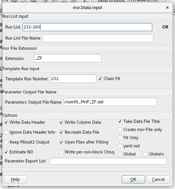
Starting will provide you a dialog looking like this:

• In the top section you can define which run numbers to analyse. In the Run List field (1) you can use space separated values and ranges, or a combination thereof. Specify there, that we want to analyse runs 232-260. You can be creative, e.g. 232 233-234 235-260. Alternatively, you can write a text file defining which runs to analyse and provide its name under (2). This is particularly helpful for reproducibility of complicated run lists. We will see an example of this later in Tutorial 6.

• In (3) we need to specify the filename of the file we want to work with, without the run-number. Since our template is called 232_ZF.msr, the Extension is _ZF.

• In (4) specify the number of your template file.

• In (5) pick a name for your the output file summarising the fit results. E.g., chainfit_MnP_ZF.dat

• For the configuration, ensure the following tick boxes are checked:

  • Write Column Data, so that you get a table-like text output

  • Recreate Data File

  • Chain Fit

  Your dialog should now look like this:

  

• Press OK to start fitting.

Musrfit will now create a .msr file for each run in the run list based on your template, try to fit it, and open it in the editor. Because Chain Fit is ticked, the starting values are taken from the previous run. This should work in this case, because the run list goes from the magnetic to the non-magnetic phase and not vice-versa. In addition, we have chosen quite strict parameter limits to keep them from running away to some nonsensical values. If you untick Chain Fit, all fits will be performed with the starting values in the template file.

Plotting the result

To see if the fit worked, we should first open each .msr file in turn and check the fit is acceptable. Once you have done this, we would like to look at the fitted paramters, which means we need to look at the output file. Since this is a comma-separated text file, you can use it to create beautiful looking figures with any software of your choice. However, if we just want to quickly know if the fitting worked, we can do so with the built-in parameter plotter.

• Start the parameter plotter using the button.

• Open the output file you just created, chainfit_MnP_ZF.dat.

• Select chainfit_MnP_ZF.dat in the list of available files, then select the dataT1 parameter, i.e. click on them so that they get highlighted.

• Click on the add X button to define the dataT1 as x-axis values. Alternatively, you can drag the parameter into the x-axis box.

• Now select the Field fit parameter and click on add Y. Once again, you can alternatively drag it into the y-axis box.

• Plot the temperature dependence of the fitted fields by clicking Plot. You can change the x- or y-axis ranges by selecting the desired range on the axis.

• If you want to look at another parameter instead, highlight Field (-0-) in the y-axis list, and press remove Y. Then add some other parameter with add Y.

Improve on the fit

The temperature dependence of the field already looks quite reasonable, and all reduced chi-squared values are close to 1. However, in the vicinity of the magnetic transition, you will see strong changes of the fractionRelax that are probably an artifact from our parametrisation.

• Go back to the template file 232_ZF.msr . (Instead of searching for it across all open files, you can also just open it again.)

• Optionally, close all other open files with Ctrl+Shift+W.

• In the template file fix the fraction to the theoretically expected value of 1/3.

  7 fractionRelax 0.3333    0        none        0       1
  

• Make sure to save the file, then open Msr2Data and run the chain-fit again.

• Plot the damping rates with , then change the y-axis to a logarithmic scale, by right clicking on the canvas: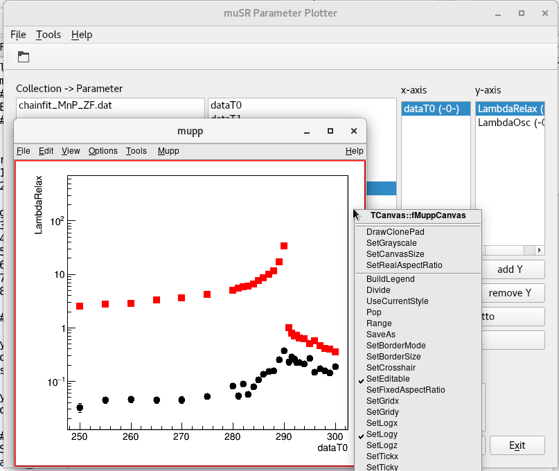

  

If you plot the other parameters, you will notice that in the paramagnetic phase, the fit is still struggling to determine Field and Phi. This is not surprising, since above 290K there are no oscillations in the spectra.

• Open the .msr files of 249_ZF.msr to 260_ZF.msr and for these, fix Field and Phase to zero, and save them (Ctrl+s):

  5 Phi         0         0           none        -20     10
  6 Field       0         0           none        0       none
  

Now, we want to use again, but without overwriting all of our manually optimised files with the template.

• Open and tick the Fit Only option. Optionally, if you want to make extra sure that your files will not be overwritten, you can also remove the Template Run Number.

• Click OK to fit all spectra again. Now the current values in each file is taken as starting value.

Manipulating individual fit files is particularly useful if only a small number of spectra did not converge correctly. Then you can adjust these, fit them by hand, and re-export the parameters with . Note that if you leave the template number field (4) empty, and have Fit Only unticked, the parameters are only exported without changing any of the .msr files.

Warning

If one of your fits did not converge, the corresponding run parameters will not be exported to the data file. Therefore, if you at some point seem to be missing one of your measurements, this is likely what happened. You would see this, for example in the STATISTIC block of the missing run, which would show:

###############################################################
STATISTIC --- 2026-01-07 15:34:24
*** FIT DID NOT CONVERGE ***

Tip

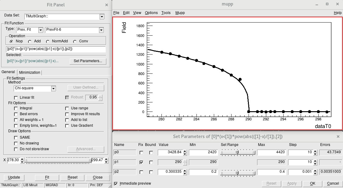
The cern root figure panel that is used by the parameter plotter is quite powerful. How to use all its functions is beyond the scope of this tutorial. Feel free to play around with it. For example, you can even use it to fit the field values to a critical scaling law:

Exercises

Exercise 1

The full ZF dataset contains lower temperatures as well, including spectra in helimagnetic low temperature phases. Have a look at these in runs 224-282 and try fitting them.

In the original publication spectra the polarisation in the helimagnetic phase was parameterised with

\[P^{\rm Hel}(t) = \frac{2}{3} e^{-\lambda_T- t} J_0(\gamma_\mu\Delta Bt) \cos(\gamma_\mu B_{\rm av} t) + \frac{1}{3}e^{-\lambda_{\rm L}t},\]

where

\[\Delta B=\frac{B_{\rm max} -B_{\rm min}}{2}\]

and

\[B_{\rm av}=\frac{B_{\rm max} + B_{\rm min}}{2}.\]

The zeroth order Bessel function of the first kind \(J_0\) is available in the THEORY block with the Bessel keyword, see documentation .

Note that an example .msr file for the 20K spectrum is available in the solution folder of this tutorial.

Exercise 2

In the next Tutorial we will learn how to do global fitting. Once you have done this tutorial, can you improve on the current analysis by globally refining some parameters? For example, Asytot, fractionRelax and potentially even Phi could be chosen to be shared across all spectra in the ferromagnetic phase.