Tutorial 4: LF and global fits

In this tutorial we will look at data measured on a highly frustrated, and thus highly dynamic, kagome antiferromagnet, Nd-Barlowite (\(\rm{Nd}_3\rm{BWO}_9\)). The corresponding measurements have been published in by A. Yadav, et al., in Physical Review B 111, 094408 (2025). You can use the data under CC BY-SA 4.0 with permission from the authors.

You have the following longitudinal field scan measured on Flame in 2022 to work with (these are some of the very first Flame measurements):

Run	T (K)	B (G)
137	87.41	40 (vert.)
139	40.00	0
140	40.00	7500
141	40.00	15000
142	40.00	22500
143	40.00	30000
144	40.00	35000

Summing histograms

The weak transverse field calibration is available in file deltat_tdc_flame_2022_0137.root.

• Use the template provided in tutorials/4.0/template/wTF_Bx_calibration_template.msr to determine the Forward/Backward alpha and beta parameters.

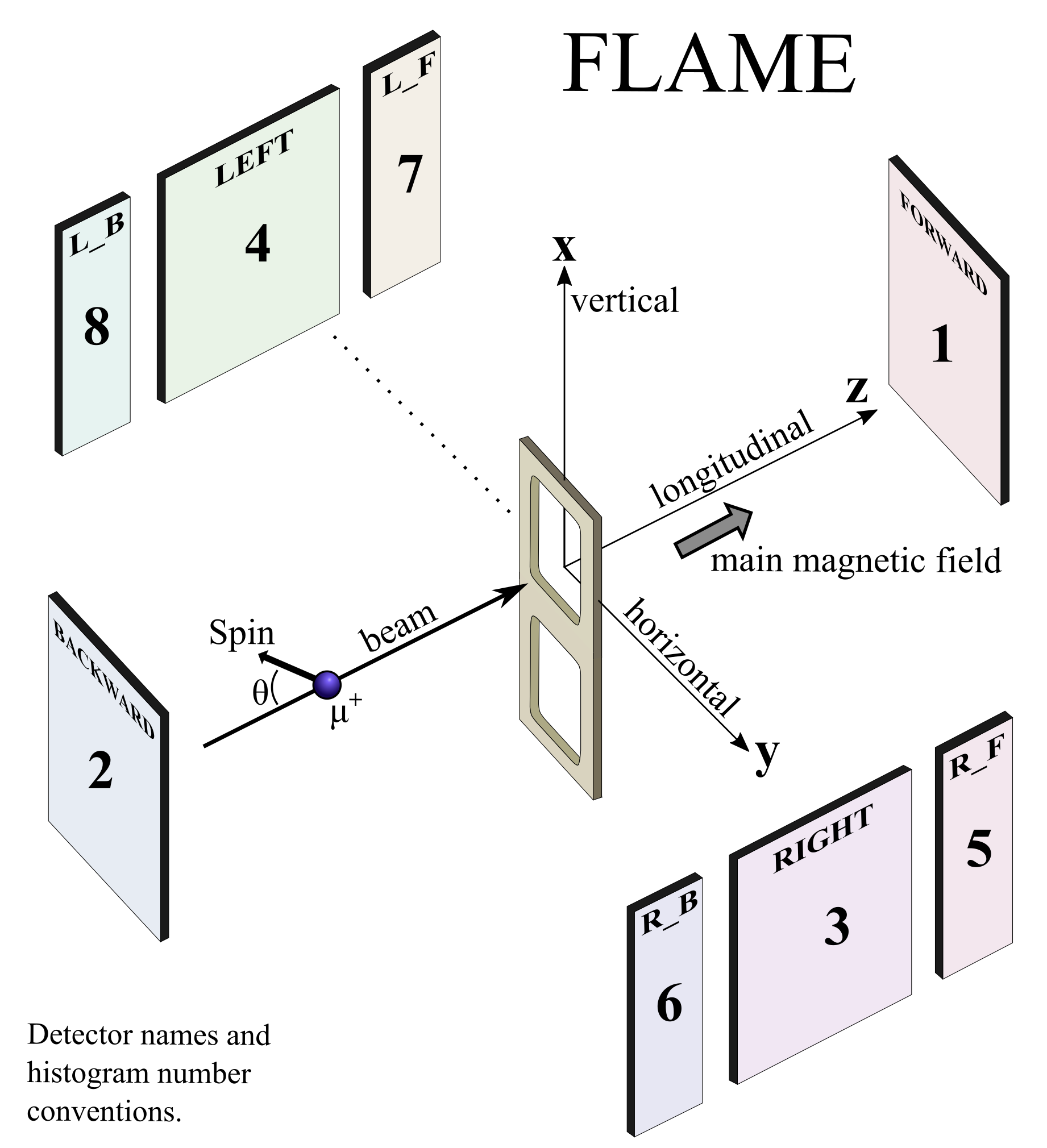
So far, we have only looked at opposite detector pairs. However, the Flame detector set is segmented, and if we want, we can add histograms from different detectors together. In particular, we can add Right_Backward and Left_Backward to Backward, and Right_Forward and Left_Forward to Forward. As you can see in the spectrometer schematic below, the corresponding histogram numbers are 6+8+2 and 5+7+1 .

Tip

The \(\mu\)SR figure of merit is \(\propto N_0 \left.A_0\right.^2\) . Therefore adding detectors to gain statistics at the cost of lowering the asymmetry is not always worth it. Similarly, in the presence of high frequencies in the spectra, any error on t0 could wash out the oscillation. In that case, analysing single histograms is preferable to summing them.

• You can add multiple histograms in the RUN block by providing lists of histogram numbers for forward and backward.

• In the first two RUN blocks for the Backward/Forward detectors, change the histogram numbers to:

  forward         2 6 8
  

  and

  forward         1 5 7
  

  Do not forget to also readjust the number of t0 values in each RUN block accordingly. Be careful, it can be difficult to correctly pick t0 when there aren’t many counts in a detector (as is the case for these smaller detectors); if you are not sure, it might be best to not use them.

  t0              1599.0  1615.0  1609.0
  

• Re-calibrate t0 . Then fit the data.

For the next part, a template file is available at tutorials/4.0/template/139_LF.msr .

• Transfer the alpha and beta values to the template.

• Reconfigure the template to use summed histograms, as we did for the wTF above. Note that it is important to always do the wTF calibration and the analysis on the same set of histograms! In theory, you can use the same t0 values as you have just got for the wTF measurements in the previous file, but it is often easier to simply redo the calibration.

  forward         2 6 8
  backward        1 5 7
  t0              1600.0  1600.0  1600.0  1600.0  1600.0  1600.0
  

• Check t0 and fit the LF template.

The next few analysis steps that follow are, in principle, not suitable for LF data. We will try them anyway so that you can get a feeling for what might go wrong…

• Fix alpha and beta by setting their steps to zero.

• Use the template to do a chain fit with , as we learned in Tutorial 3, and look at the resulting field dependence with .

You will notice a very strong field dependence on the asymmetry.

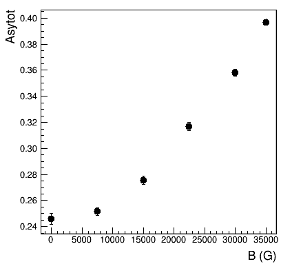
Such high values for the asymmetry are not realistic on Flame. Therefore, we must have made a mistake in our analysis of the data. In particular, a high longitudinal field will focus the incoming muon beam, and highly affect the positron tracks. In 3.5 T, we expect a cyclotron radius for the highest energy decay positrons of about 5 cm. Therefore, the geometrical acceptance of the asymmetrically placed forward and backward detectors will change as a function of field. In our data analysis, we should thus assume alpha to be field dependent. We cannot do much about beta, because we cannot fit it in an LF geometry, so we will continue having it fixed. This is usually not much of a problem, since the field dependence of alpha is much more pronounced.

Generating global files

Now, we could just fix the initial asymmetry and do a chain fit refining alpha. However, what we would rather do is still fix alpha for the lowest field measurement, and then refine the value of the asymmetry shared for all measurements.

First, we need to adjust our template file in order to specify which parameters will depend on the run number. Note this is different from mapping, as you can do this with single histogram fits that have multiple mapped RUN blocks for the same run number.

• Declare alpha and the two relaxation rates to be fit individually, by appending a four-digit _RunNumber to the parameter names. Also, release alpha by giving it a finite step size:

  1 alpha_ForwBackw_0139    1.0078    0.1         none
  2 beta_ForwBackw          0.9046    0           none
  3 Asytot                  0.2461    0.0042      none
  4 fraction                0.86      0.1         none        0       1
  5 LambdaFast_0139         5.75      0.33        none        0       none
  6 LambdaSlow_0139         0.712     0.044       none        0       none
  

• We can now generate a global fit file with . Simply tick Global and Create-msr-File-only. Then confirm with OK.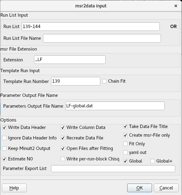

  

  This will generate a file 139+global_LF.msr that has your shared parameters on top, and the specific parameters listed below. Note that you may need to open the file manually if it does not automatically do so.

• In the PLOT block, specify to plot all runs with:

  runs     1-9
  

  You can now look at all runs together with . Of course, without fitting, the data will still be offset.

Initialising Global fits

The current example is simple enough. So we could just fit it and would immediately achieve convergence in a reasonable time. However, for more complicated global fits, this might not be the case. There are a couple of tricks to deal with this problem.

An easy solution is to first fit each run individually, before constructing the global file. This can be achieved with the Global+ option in .

• It is often a good idea to first fix all shared parameters to a value that you expect might be a good value, e.g. based on the results of individual fits. This prevents individual parameters from running away. In this case, in the template file 139_LF.msr set the step of Asytot to zero:

  3 Asytot    0.2461    0.        none
  

• Re-run as before, with Create-msr-File-only. This time use Global+ instead of Global.

As you see, this will automatically create a file RUNNUMBER-OneRunFit_LF.msr for each run, fit it and then automatically paste the resulting parameters into your global file.

Hint

The RUNNUMBER-OneRunFit*.msr files will be re-generated based on the template whenever you do a new Global+ fit. There is usually no point in looking at them, or modifying them.

• Open the resulting 139+global_LF.msr global file if it does not show up automatically. If you have it already opened, you might want to refresh it to ensure it is up to date.

• In the global file, fix the alpha value of the zero field run 139 to the value you found with the weak transverse field calibration.

  # Specific parameters for run 139
    4 alpha_ForwBackw_0139      1.0078     0         none
  

  This will ensure the shared asymmetry will stick to reasonable values. If you later notice that the fit is well behaved without this measure you can consider releasing the parameter again.

• Release the asymmetry by giving it a non-zero step.

Another trick we can try to improve convergence is to now refine only the shared parameters first before fitting everything.

• Adjust your command block, to first only fit the asymmetry, and then everything together. You can use FIX number/name and RESTORE to fix individual parameter numbers/names and afterwards release them again.

  ###############################################################
  COMMANDS
  FIX 3 4 5 6 7 8 9 10 11 12 13 14 15 16 17 18 19 20
  MIGRAD
  HESSE
  RESTORE
  MIGRAD
  HESSE
  SAVE
  

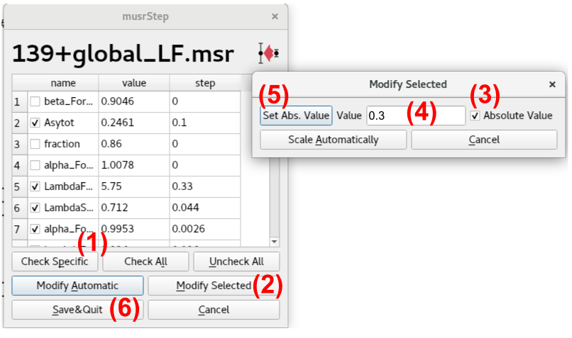
One problem that often occurs, especially if you do not use Global+ initialisation, is that your fitted template or your OneRunFits significantly underestimate the error and you would need a larger step-size to achieve convergence. There is a button Set Steps that allows you to automatically modify a large number of steps.

• Click on . Then Check All, to select all parameters that have not been fixed.

• Use Modify Selected, check Absolute Value, give an appropriate starting step, e.g. 0.3, and update the steps pressing Set Abs. Value.

• Confirm the new steps by pressing Save&Quit.

  

Warning

Be careful with the Scale by Factor and Modify Automatic: if some of your parameter values currently happen to be zero these will be fixed instead of being given an appropriate step.

• Finally, complicated global fits might run into the default timeout of one hour. To change it, open Preferences . Then change the default timeout to two hours by specifying 7200 as a timeout value in the general tab.

• Fit the global file and plot the result. You will probably need to update the PLOT block again, to show all runs 1-9.

Tip

Another trick to improve convergence is to set reasonable parameter and error values. If in doubt, something with an order of magnitude of one usually works quite well.

For example, in a transverse field file the following parametrisation will struggle to fit exact field values:

   1 Phi         0           1           none
   2 Field       34602.8385  0.00012     none
THEORY
TFieldCos      1  fun1    (phase frequency)
FUNCTIONS
fun1 = gamma_mu * par2

A much better and equivalent parametrisation in this case would be:

   1 Phi            0           1       none
   2 Field_Fixed    34602.83    0       none
   3 Field_Offs_mG  8.5         1.2     none
THEORY
TFieldCos      1  fun1    (phase frequency)
FUNCTIONS
fun1 = gamma_mu * ( par2 + par3 / 1000 )

As both fitting parameters 1 and 3 now have a similar magnitude and step size, you can expect the fitting algorithm to be more stable.

Export data from a global fit

To analyse the field dependence of the fit parameters, you will want to export and visualise the results of the global fits. Similar to how we did this when chain fitting, we can use and for this purpose.

• Open .

• Ensure that there is no Template Run Number . This is important, otherwise your global fit file might be overwritten!

• Tick Global, Write Column Data, Recreate Data File, and provide a proper name as Parameters Output File Name.

  

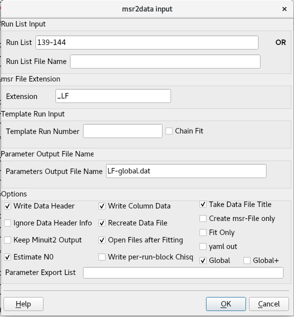
• If you want to fit again before exporting the parameter values, tick Fit Only.

• After confirming with OK, a data file will be created. The format is exactly the same as for non-global fits, so you can plot it with or some other software of your choice, the same as before.

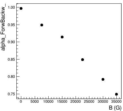
Looking at the results of this global fit you can see that, as assumed, the initial asymmetry is field independent. Conversely, the relaxation rates are field dependent. Alpha shows a strong and systematic field dependence which reflects the change of positron tracks in the applied field :

In tutorials/4.0/solution you will find an example of how your global fit file 139+global_LF and your template file 139_LF.msr might look.