Tutorial 6: Meissner state

In this tutorial, we will analyse Meissner state measurements on a superconductor measured with low energy muons. You will learn how to use run list files, and how to fit ascii raw-data.

The sample we will look at is a 2x2 cm² thin film of the prototypical high temperature superconductor YBCO with a layer structure of \(\mathrm{ 10nm CeO_2 / 300nm YBa_2Cu_3O_7 / LaAlO_3}\).

The following dataset is at your disposal, with the raw data being located in data/lem22_his_1281.root.

Run	T (K)	B( G)	Energy (keV)	Range(nm)
1281	10.00	96.7	22.06	99.4
1282	10.00	96.7	18.76	84.1
1283	10.00	96.7	15.37	69.9
1284	10.00	96.7	12.06	56.5
1285	10.00	96.7	8.77	43.5
1286	10.00	96.7	5.37	30.8
1287	10.00	96.7	2.61	19.4
1309	100.00	96.7	22.06	99.4
1310	100.00	96.7	18.76	84.4
1311	100.00	96.7	15.37	69.9
1312	100.00	96.7	12.06	56.5
1313	100.00	96.7	8.77	43.5
1314	100.00	96.7	5.37	30.8
1315	100.00	96.7	2.07	17.3

The average range of the muons in the last column was estimated using Trim.SP.

Run lists

Open the template file tutorials/6.0/template/1281_shist.msr.
Do the usual checks to verify that the fit is alright. , , , and (see Tutorials 1 and 2). Note that, as we are adding two detectors per histogram, the t0 estimation and data selection happen in sequential order, rather than simultaneously.

You might note the following peculiarities compared to previous tutorials: we are using a single histogram fitting with logarithmic likelihood maximisation, because sometimes spectra on LEM have a time dependent background. Moreover, instead of the left/right spectra in histograms (1, 5 / 3, 7) we are using histograms (21, 25 / 23, 27). Those are based on the same detectors but include a rejection of post-pile-up positrons. (Due to the low event rate, LEM is the only PSI instrument that does not use post-pile-up rejection by default.)

Create a new text file , with the following content and save it as runlist-10K.txt in the same folder as the .msr file:
```
RUN  RANGE
1281 99.4
1282 84.1
1283 69.9
1284 56.5
1285 43.5
1286 30.8
1287 19.4
```
Note that the second column is optional, but it ensures that the result from our TrimSP will be included in the output file by Msr2Data .

Use to do a chain fit of the 10 K dataset (see Tutorial 3). You can use run 1281 as a template file and write the results as a column data file into 10K-Escan.dat. However, this time, instead of writing run numbers into Run List, use the runlist-10K.txt file in the Run List File Name field:
Verify that your fitting was successful, i.e. check the fits, maxLHred and the fitting parameters with (Tutorial 3).

Fitting text-based raw data

Open the 10K-Escan.dat output text file to inspect at it. (If you only see .msr files in the file open dialog, note that you can switch to showing all files at the bottom right.)
In the top header line, count the parameter column indices, ignoring all names ending with Err. So, RANGE is parameter number 8, and Field is parameter 17 .

Write a new .msr file to fit the 10K-Escan.dat output file. We can use 8 as value for fittype and PLOT to analyse ascii data. If you generated your data-file with msr2data and ticked Write Column data, the appropriate data-file-format you need to specify in the RUN block is DAT. To fit Field as a function of RANGE, we need to provide the column indices from above in the run block: xy-data 8 17.

###############################################################
FITPARAMETER
###############################################################
      1 Field       100       0.1       none
###############################################################
THEORY
const          1
###############################################################
GLOBAL
fittype         8         (non muSR fit)
fit             0       1000
packing         1
###############################################################
RUN 10K-Escan.dat MUE4 PSI DAT   (name beamline institute data-file-format)
xy-data         8       17
map             0    0    0    0    0    0    0    0    0    0
###############################################################
COMMANDS
MIGRAD
HESSE
###############################################################
PLOT 8   (non muSR plot)
runs        1
range    0   150

Verify that you can calculate chi-squared and plot the data.

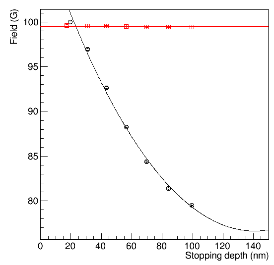
Meissner screening

In an infinitely thick superconductor, when assuming a local response, the magnetic fields at the surface are screened exponentially from the interior. The corresponding length scale is the London penetration depth \(\lambda_\mathrm{L}\).

We expect that the \(\mathrm{10nm CeO_2}\) layer will cause a non-superconducting dead layer \(d_\rm{d}\) on top of your sample. So, as a simplified first attempt, we can try to fit the Meissner screening as a function of depth \(z\) with:

\[B(z)=B_0 \exp\left(-\frac{z-d_0}{\lambda_\mathrm{L}}\right).\]

Adjust your FITPARAMETER, THEORY and FUNCTION block to implement this function. Note that we implicitly assume that all our measured points are inside the superconducting layer:

###############################################################
FITPARAMETER
###############################################################
#    No Name        Value     Step        posError  [Lower_Boundary Upper_Boundary]
      1 Bext        96.7      0           none
      2 LambdaL     20        0.1         none
      3 dead_layer  10        0.1         none

###############################################################
THEORY
const          1
const       fun1
simplExpo   fun2          (rate)

###############################################################
FUNCTIONS
fun1 = exp(par3 / par2)
fun2 = 1 / par2

As you see, with the simplExpo we can use all previously used theory functions. In the THEORY block, the variable that we specified as x in the RUN block takes the role of the time. Whereas in the function block, we can define auxiliary functions of the parameters, but only if they do not need the x variable.

If you now fit the data, you will find that our model does not describe the data very well.

There are several reasons for the poor fit quality. First, we have not yet determined our applied field, which might be different from the nominal 9.67 mT. Second, we are measuring a thin film, and the London penetration depth is significant compared to the film thickness \(d_{sc}\). Finally, we are not measuring at a fixed depth, but instead, the low energy muon stopping profiles typically have a width on the order of 10nm.

Fit the data at 100K above the superconducting transition temperature.
Include the resulting data file as an additional RUN block in the file where you analyse the depth dependence. Share the Bext value of both datasets.

If we assume the field penetrates from both sides into the superconductor, the depth dependence inside the superconducting layer becomes

\[B(z)=B_0 \frac{\cosh\left((d_{sc}/2-z)/\lambda_\mathrm{L}\right)}{\cosh\left(d_{sc}/(2\lambda_\mathrm{L})\right)}\]

Adjust this formula to include a dead layer. Then implement it in your fitting file. Note that you can use hyperbolic cosines in the function block, but not in the theory block. Therefore, you have to express one of them as two exponentials. Although still not perfect, the resulting fit should be much better than before:

If you need help, look at the solution in tutorials/6.0/solution/Meissner.msr.

Hint

If you want to fit more complicated functions with musrfit, it is recommended that you write and compile your own user function. For the Meissner state some are already available if you install musrfit with BMW-libs enabled. They calculate the time spectra by convoluting the Trim.SP stopping profiles with the Meissner screening field profile. Using them is beyond the scope of this tutorial, but you can find their documentation and the syntax of how to declare them in the THEORY block here.