Tutorial 2: Single Histograms

Up until now, we have looked at asymmetry spectra, which are proportional to the ensemble average of the muon spin direction along a certain detector axis. Given two detectors, the asymmetry is obtained by looking at the normalised difference between the two histograms. However, in some cases, it is of advantage to instead analyse only an individual detector. In musrfit we call this single histogram fitting, and this tutorial will show you how to use them.

Single histogram fitting

Open the template file tutorials/2.0/template/804_shist.msr

Can you spot the differences to the previous asymmetry fit?

A single histogram fit is declared by changing the fit type from 2 to 0

###############################################################
GLOBAL
fittype         0         (single histogram fit)

In addition, the same needs to be specified for plotting

###############################################################
PLOT 0   (single histo plot)

There are also some more subtle differences: Instead of alpha, we are fitting the initial number of counts \(N_0\) and a background \(N_{\rm bkg}\). Like alpha before, these are defined in the Run block. Also note that for single histogram fitting, we can only specify a forward but no backward detector:

###############################################################
RUN deltat_tdc_flame_2024_0804 PIM3 PSI MUSR-ROOT   (name beamline institute data-file-format)
norm            1
backgr.fit      2
forward         2

Set proper t0 and data ranges . Note that you do not need to set the red background range, since it will be ignored (and later fit) anyway.

You might have noted by now, that the resulting data range is rather large. This is because the spectrum we are looking at was measured with a 20 \(\mu\)s data gate. In order to fit and plot the full data range, we can adjust this in the GLOBAL and PLOT blocks. Change the fit range to
```
fit             0.01    20
```
and the plot range to
```
plot_range 0 20
```
Fit and plot the data. Remember by pressing t on the plot window you can change the fit line colour.

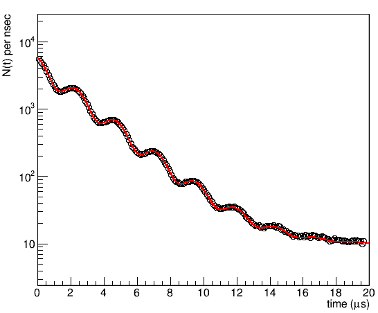
This is what a single histogram spectrum looks like. What you see at early time is an exponential decrease of the spectrum due to the radioactive decay of the muon with a lifetime \(\tau_\mu\sim2.2 \mu s\). At late time the spectrum flattens off to a constant value given by the uncorrelated background. On top of that the spectrum is modulated by the weak transverse field oscillation.

We can describe the functional form of the spectrum as:

\[N(t) = N_0 e^{-t/\tau_\mu} [ 1 + A(t) ] + N_{\rm bkg}\]

Here the asymmetry \(A(t)\) describes the decay asymmetry we looked at previously and corresponds again to the function you can define in the THEORY block.

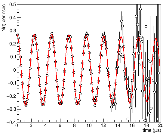
Small details in the asymmetry can be hard to spot in a raw spectrum, and most people are not very used to looking at it. Therefore, it is often helpful to solve the equation above for the asymmetry and plot this instead, i.e.

\[A(t) = \frac{N(t) - N_{\rm bkg}}{N_0} e^{+t/\tau_\mu} - 1 .\]

To do so, replace the logy keyword with lifetimecorrection in the PLOT block. Note that this only affects how we visualise the data.
```
PLOT 0   (single histo plot)
runs     1
#logy
lifetimecorrection
```

If you plot the data now, it is immediately obvious that the fit quality is poor at very late times. This is a known issue with a chi-squared minimisation in combination with low statistics data. To improve the fit, we can instead maximise the logarithmic likelihood.

Do so, by adding the MAX_LIKELIHOOD keyword to the COMMANDS block
```
###############################################################
COMMANDS
MAX_LIKELIHOOD
MIGRAD
HESSE
```
The other keywords can remain unchanged. MIGRAD specifies the minimisation algorithm, and HESSE the error estimation.
If you now fit the late-time fit-quality is significantly improved:

Adding spectra

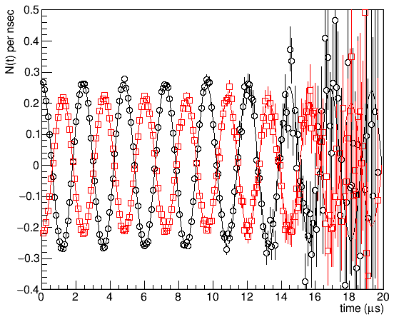
If we only analyse a single spectrum, we ignore half of the measured information, compared to analysing an asymmetry fit. Therefore, we should add the second detector. We can do this, by duplicating the previous run block, and replacing the number of the analysed histogram provided with the forward keyword from 2 to 1.

Change the run blocks to the following. (You can either take the t0 value from the previous tutorial, or rerun the t0 calibration.)

###############################################################
RUN deltat_tdc_flame_2024_0804 PIM3 PSI MUSR-ROOT   (name beamline institute data-file-format)
norm            1
backgr.fit      2
forward         2
map             0    0    0    0    0    0    0    0    0    0
t0              1618.0
data            1642    203152

RUN deltat_tdc_flame_2024_0804 PIM3 PSI MUSR-ROOT   (name beamline institute data-file-format)
norm            1
backgr.fit      2
forward         1
map             0    0    0    0    0    0    0    0    0    0
t0              1628.0
data            1652    203152

You should now be able to plot musrview the second spectrum by adding to the plot block as below, but you will immediately notice that the fit function is wrong.

PLOT 0   (single histo plot)
runs     1   2
#logy
lifetimecorrection

First, let us try to fit the second spectrum completely independent of the first one. The trivial way to do this, would of course be to just change the detector number in forward instead of duplicating the run block. But then we could not share some parameters afterwards.

Duplicate the parameters. Ensure the numbering is correct and that names are unique. E.g.:

FITPARAMETER
###############################################################
#  No Name         Value     Step        posError
N0_B         4448.0    1.1         none
Background_B 10.285    0.029       none
Asymmetry_B  0.27012   0.00036     none
Sigma_B      0.0256    0.0027      none
phi_B        2.53      0.11        none
Field_B      30.5744   0.0072      none
N0_F         4448      1.1         none
Background_F 10.285    0.029       none
Asymmetry_F  0.27012   0.00036     none
Sigma_F      0.0256    0.0027      none
phi_F        2.53      0.11        none
Field_F      30.5744   0.0072      none

In the RUN block, change norm and backgr.fit for the second run to parameters 7 and 8 respectively.

The other parameters we have to redirect in the THEORY and FUNCTIONS blocks. There, we can make a parameter RUN block specific, by specifying mapN instead of a parameter number. Then, the parameter number will be looked up at the N^th position of the map list in the RUN block.

So for example, if we change

THEORY
asymmetry      map1

we can then use

map             3   0    0    0    0    0    0    0    0    0

and

map             9   0    0    0    0    0    0    0    0    0

respectively, to encode the asymmetry in parameter 3 for the first run and in parameter 9 for the second run. Similarly, we can replace parN by some mapN in the function block.

Replace all parameter numbers by maps.
Try fitting the data.

If you struggle, you can have a look at the file tutorials/2.0/solution/804_shist_1.msr

Hint

Instead of adding a second RUN block and changing the detector, you can also add a second run block and change the file name. Like that you can analyse multiple measurements simultaneously. Of course, writing such files with many runs becomes cumbersome very quickly. In Tutorial 4, we will generate them automatically for a large number of measurements.

Shared parameters

On a conceptual level, there is no reason for the Field or the damping Sigma to depend on the detector. Indeed, you will see that their values are almost the same.

If you want to share these parameters across both run blocks, simply undo the mapping again for those two parameters, or map them to the same number. (An example how this might look like is in tutorials/2.0/solution/804_shist_2.msr.)

alpha and beta geometric parameters

If we look at the FITPARAMETER block, you will notice that not only are the phases of the two detectors about 180° different, but also the values of \(N_0\), \(N_{\rm bkg}\), and \(A_{0}\) vary significantly. Enough that you can see it by eye if you compare the raw- and lifetime-corrected spectra.

This is due to the detector geometry. In general, the detectors might not have the same efficiency, and samples are sometimes mounted off-centre. For the FLAME spectrometer in particular (where these data were measured), the actual placement of the forward/backward detectors is asymmetric to begin with.

Comparing this to an asymmetry fit, if we declare the spectrum \(N_\rm{f}(t)\) to be forward and \(N_\rm{b}(t)\) to be backward, then we can define the following two geometrical ratios:

\[\alpha = N_{0,\rm{b}}/N_{0,\rm{f}}\]

and

\[\beta = A_{0,\rm{b}}/A_{0,\rm{f}}.\]

When doing asymmetry fits, both of these parameters need to be accounted for. To calculate the asymmetry based on the two raw spectra, one can use:

\[A(t)=\frac{\alpha\left[N_{\mathrm{f}}(t)-N_{\mathrm{bkg,f}}\right]-\left[N_{\mathrm{b}}(t)-N_{\mathrm{bkg,b}}\right]}{\alpha\beta\left[N_{\mathrm{f}}(t)-N_{bkg,\mathrm{f}}\right]+\left[N_{\mathrm{b}}(t)-N_{\mathrm{bkg,b}}\right]}.\]

In asymmetry fits, you can assign parameter numbers to alpha and beta in the RUN block by using the alpha and beta keywords.

Warning

In an asymmetry fit, if the alpha parameter is chosen wrong, the spectrum is offset. (As we saw in Tutorial 1.) That is why we can easily calibrate it with a weak transverse field on a paramagnetic/diamagnetic sample. On the other hand, the systematic error from using an incorrect beta is significantly smaller. In many cases, it is alright to assume \(\beta=1\), which is the default chosen if no beta keyword is present in the RUN block. However, you should be aware that if beta is very far off, it can cause artifacts like higher harmonics in the spectrum. Because beta is strongly correlated with the initial asymmetry, it cannot reliably be refined with an asymmetry fit. So you should only ever try to fit it with single histograms.

We will now use what we have learned so far to parameterise our single histogram fit file in terms of alpha and beta fitting parameters. This should not add new fitting parameters, only reshuffle them.

Prepare the FITPARAMETER block by renaming 7 N0_F to 7 alpha and 9 Asymmetry_F to 9 beta. In addition, change their values to 1 to have a reasonable starting guess.
Introducing alpha is rather straight forward: In the second run block have norm point to fun2
```
norm            fun2
```
which you define as N0_B * alpha
```
fun2 = par1 * par7
```
To parametrise as a function of beta, we need to change the asymmetry line in the THEORY block. Clearly, a simple mapping will not do the trick. Lets delegate the problem to another function:
```
asymmetry   fun3
```
We want fun3 to be par3 in the first runblock and par3 * par9 for the second. We can achieve this by introducing an additional parameter that is always fixed to 1. Therefore,
```
fun3= par3 * map1
```
using a fixed parameter (your numbering may be different, depending on whether you are sharing B and sigma between the two detectors or not)
```
11 ONE         1         0           none
```
where in the first RUN block we now have map1 resolve to ONE, and in the second to our beta parameter.
After fitting, you should find that alpha is very similar to the value from the first tutorial. As expected for this measurement, beta is not well approximated by 1.
You can find an example of how your final file form this tutorial might look like in tutorials/2.0/solution/804_shist_23.msr.